This is a continuation of my previous post where I looked at filtering variants in rare disease trios.
In building out slivar, I have largely focused on trios–where mom, dad, and affected kid are present. I assumed that with only a single affected sample, it would substantially reduce the solve-rate and increase the false-positive rate, in which a ostensibly causal variant was mis-categorized or leave so many candidate variants that the solve-rate would be lowered.
A recent Cell paper looked at > 2200 Saudi families where a proband had rare disease. The apparent solve-rate was no different for singleton samples than for trios; this could be due to the choice of when trio-sequencing was needed, but, still, interesting. Also, Harriet, who has just joined the Quinlan lab, is co-author on a paper that, evaluates singleton exomes and finds that gene-lists created by clinicians facilitate variant prioritization.
I ran an in silico experiment where a set of high-quality candidate variants is found with each of 149 trios with exome sequencing. Then each family is computationally reduced to a duo–with only 1 parent, and then a solo, with just the proband.
Without a team of clinicians, one can’t know the true causal variants, even with trios, but the solo analysis should be able to recover a superset of the variants from the trio analysis. As that superset becomes too large, it becomes less plausible that solo sequencing is a viable analysis strategy. This is imperfect, but can give a general idea of the task.
This analysis includes de novo, single-site, autosomal recessive, x-linked recessive, and compound heterozygote inheritance patterns. slivar has been updated to better support duo and solo families with the latest (pending) release.
The filtering is on only:
- inheritance pattern
- depth
- genotype-quality
- allele-balance
- gnomAD allele frequency
For example, the filters for de novo variants are:
- trio:
$HQ && mom.hom_ref && dad.hom_ref && kid.het && kid.AB > 0.2 && kid.AB < 0.8 - duo:
$HQ && mom.hom_ref && kid.het && kid.AB > 0.2 && kid.AB < 0.8 - solo:
$HQ && kid.het && kid.AB > 0.2 && kid.AB < 0.8
where $HQ ensures that each sample has depth >= 7 and GQ >= 10 and that variant.FILTER == 'PASS' and the variant is at a low allele-frequency (0.001 for de novo and 0.01 for recessive) in gnomAD. Below is the result of counting the number of variants that pass filters for each inheritance mode for 149 trios, from which we also create 149 duos (kid, mom) and solos (just kid).
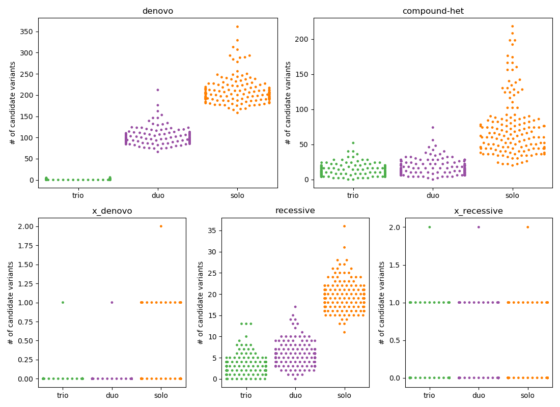
In the plot above, each point represents a proband with the y-position being the number of passing variants and the color indicating trio, duo, or solo, each subplot is a different inheritance mode.
I have placed denovo and compound-het on the top row because these are the 2 modes where the number of candidates for solo is too high to be feasible. For other inheritance modes, the number is quite reasonable.
Additional Filtering for solo de novo and compound-het
200 variants, as in the case of solo de novo in the plot above seems too many to reasonably evaluate, we can reduce this number by:
- limiting to functional variants
- lowering the gnomAD allele-frequency thresholds
- raising depth and genotype-quality thresholds
- filtering on TOPmed allele-frequency
- limiting to genes of interest
of those, the last is the most difficult as it requires either knowledge of the phenotype in each of the 149 probands or trust in a gene-wide score such as pLI or gene-damage-index. We can, however, limit to a set of genes previously associated with (any) disease using this file which uses OMIM disease annotations.
In order to limit to “functional variants”, I used only variants with a variant-effect-predictor VEP of MODERATE or HIGH. This includes missense variants, so it is still pretty permissive.
Compound heterozygotes in solo samples
The number of compound heterozygotes in a single sample could be reduced to an average of 21 candidate variants (so 10-11 genes) by requiring functional variants with 1 or fewer homozygous alternates in gnomad controls and limiting both the topmed (via dbsnp) and gnomAD popmax allele frequency to < 0.005. Since this number was low enough with strict, but sane filters, I did not explore further filtering for compound heterozygotes.
De novo in solo samples
Since a putative de novo variant in a solo analysis is simply a high-quality, rare heterozygote, the findings here will also translate to autosomal dominant since that would have the same constraint. The starting point here is about 200 variants per sample, as shown by the cluster of orange points in the top-left (de novo subplot from the figure above. Here, I’m not (currently)recommending a best-practices approach, just exploring the possibility of reducing this to a more reasonable number of candidate variants.
The plot below shows the number of candidate “de novo” variants in a solo sample.
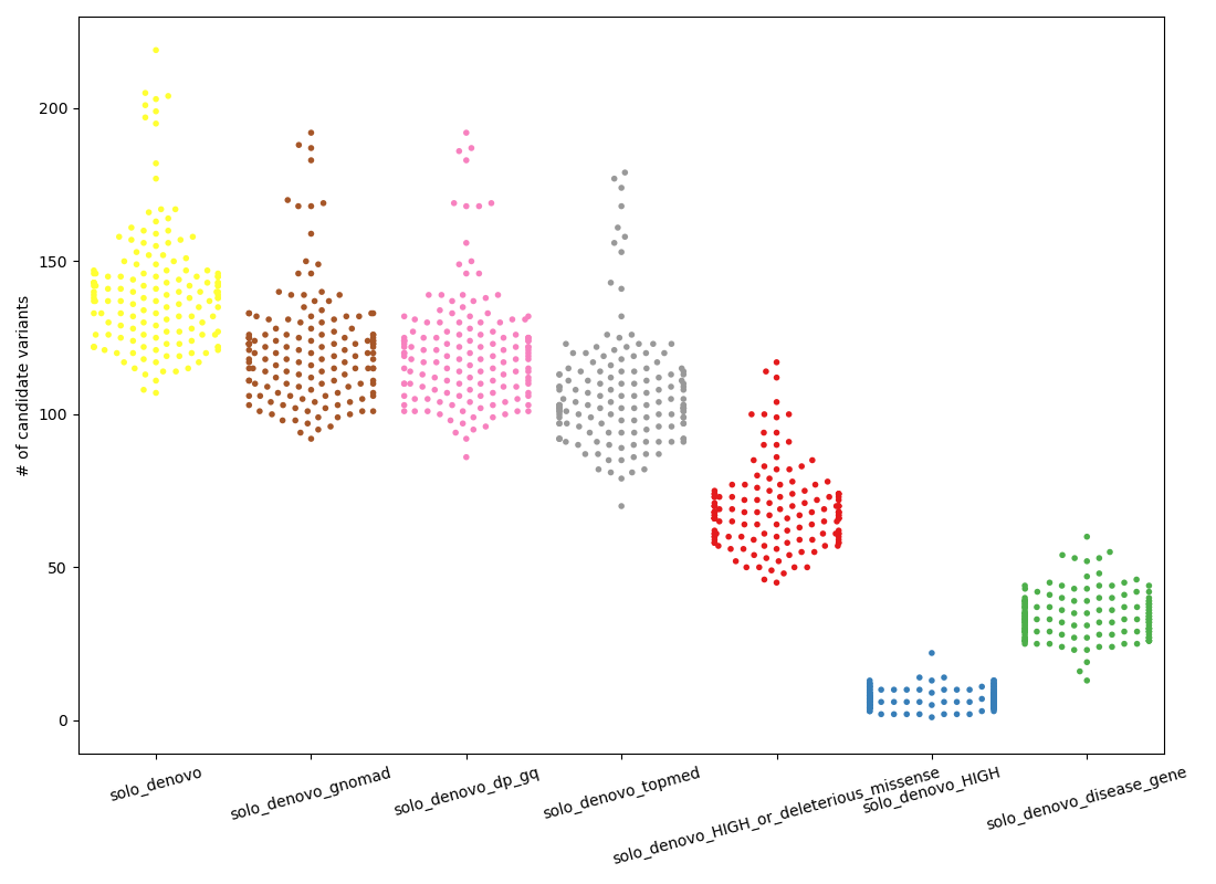
Except for the final column, each column along the x-axis is a more stringent subset of the one that precedes it. The left-most column, in yellow continues from the orange cluster in the de novo subplot of the first figure by requiring, from left-to-right:
solo_denovo(yellow):HIGHorMODERATEimpact according to VEPsolo_denovo_gnomad(brown): frequency in gnomad controls < 0.005 and number of hom-alts in gnomad <= 1solo_denovo_dp_gq(pink): depth > 10 (was depth > 6)solo_denovo_topmed(gray): frequency in topmed < 0.02 (can catch problems with lifting gnomAD to hg38)solo_denovo_HIGH...(red): impact is HIGH according to VEP or the variant is missense and has a sift score or polyphen score that predicts it to be damaging/deleterioussolo_denovo_HIGH(blue): impact is HIGH according to VEPsolo_denovo_disease_gene(green): the variant exists in a gene associated with some disease in OMIM. this is a subset of the gray column.
The final (green) column is a subset of the gray column; it shows an alternative strategy that looks at gene, rather than at the function of variants (as in red and blue).
Intuitively, the red and green columns seem the most reasonable balance of stringency and likely recall. For example, we are unlikely to solve a rare-disease case if the variant is not MODERATE or HIGH impact accordign to VEP. At a mean of about 70 and 35 variants per sample, respectively, these are not ideal, but 35 is a number of variants that a clinician or analyst could reasonbly evaluate.
Note that the drop from pink to gray indicates the effect of using TOPmed annotations that are not visible in GRCh37 but common (at more than 2% allele frequency) in hg38.
Conclusions
- It is possible to recover a small candidate-set by applying minimal filters to a parent-child duo. To me, this is the most useful result of this analysis which I think is also a novel observation.
- For a solo (singleton) sample, given the number of candidate variants, it is unlikely to “solve” a de novo or dominant case without prior knowledge–for example a small set of genes of interest. This will be unsurprising to most, still the analysis in the 2nd figure above does show how much the set of candidate variants can be reduced.
- For a solo sample, it does seem possible, based on the number of candidate variants to solve a recessive case–either a single-site autosomal recessive or a compound heterozygote.
- Due to dark regions, variants that are common in hg38 are completely absent in GRCh37 so lifted gnomAD annotations will not filter some common variants. The shift from pink to gray in the 2nd figure shows this; the reduction (after previous filtering) is ~10-15%.
Thanks to Harriet, Aaron, Amelia, Matt and Jessica for feedback on these analyses.