Indexcov: cover your bases

This post is to introduce indexcov and answer common question I get about interpretation.

I have found that, as indexcov is applied to cohorts approaching size of 100 or so, the probability that it will reveal something very interesting (either a data artefact or large chromosomal anomaly) approaches 1.0. For example, who knew that there were trisomies in Simons diversity panel?

indexcov quickly estimates coverage for whole genome BAM and CRAM files. It takes about 1 second per BAM. It does this by not parsing the BAM, instead, it uses the linear index in the BAM index. The BAM index contains a “linear index” that, indicates the file offset (in bytes) for every 16384 bases in the genome. indexcov relies on the assumption that the the difference in file consecutive file-offsets in the index (which indicates the amount of bytes within a 16KB region) is a reasonable proxy for the coverage in that 16KB region. It does some other sourcery for CRAM index files.

There are many reasons this coverage estimate can be wrong. Some of those reasons are enumerated in the indexcov paper. In practice, it seems to work. Internally, indexcov will normalize each 16KB bin to the median, so bins with “normal“ coverage will have a value around 1. Calculating this normalized coverage (and then doing a PCA) is most of the computational work that indexcov performs, the rest is visualization.

Given a command like (yes, it’s this simple):

goleft indexcov -d output/ path/to/*.bam

output/index.html will show a number of plots; some are interactive and some are static images that can be clicked to go to an interactive plot.

To orient, here is X chromosome, where we expect males to have a coverage of about 0.5 and females about 1 (since everything is scaled to 1 for diploid copy).

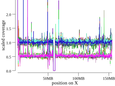
The x-axis is position along the chromosome, and the y-axis is scaled coverage. This cohort has 50 so samples all shown in the same plot, each sample with it’s own color. Note we can clearly see the group of females at coverage of 1 and males at 0.5. There’s a gap in coverage at the centromere and some large variation, including at the start of the chromosome.

In the index.html, indexcov shows this plot as a static png, which, when clicked, takes the user to an interactive version that allows hovering to see per-sample info.

indexcov makes a similar plot for the Y chromosome where, again, males and females separate cleanly. It then uses the data from the sex chromosomes to make a plot like this:

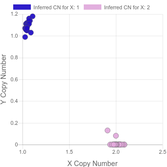
Note that, among other uses, this type of plot helps to find XXY samples which are not detectable when looking at X and Y in isolation.

In a recent project, we saw this:

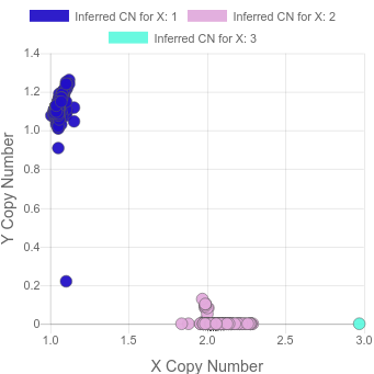
where there’s a sample with 3 copies of X and another sample where most cells appear to have lost the Y.

It’s also possible to see large (>10MB deletions). For example, here’s a deletion at the end of chr10 found in a cohort of 1200 samples:

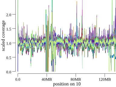
It takes a couple of seconds of concentration to see it, but this is 1200 samples, so we can scan an entire genome for large events in a couple of minutes. These are the types of events that would be embarrassing to miss, but, in fact, they are easy to miss unless you have a pipeline doing much more expensive LOH or coverage analyses. Even depth-based CNV callers have trouble with events like these.

Here’s another example of the Angelman deletion at the start of (acrocentric) chromosome 15 in a cohort of 45 samples:

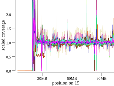
Another way to plot this is a cumulative coverage plot. The same plot above can be seen somewhat more concisely as

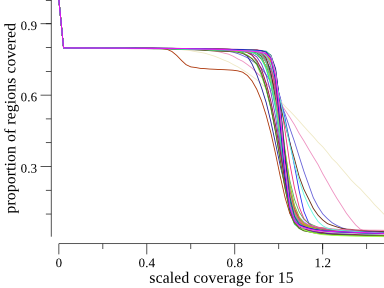
Since much of the chromosome is not covered due to the acrocentric chromosomal region, the y-axis starts at about 0.8 for all samples. For most samples, it does not drop until about 1. This means that most samples are covered at about 1X for 80% of the genome. We can see the angelman sample because it drops earlier, plateau’s, and then meets up with the rest of the samples around one. This plot is a more concise way to show the data. It appears side-by-side with the depth plot in the HTML output of indexcov.

Bin outliers

One thing we can see from the plots above for chromosome 15 is that some samples are frequently farther from the expected coverage of 1. For those plots, the offending samples are pink and light tan colored. These also appear as the samples with the least vertical lines as the pass through a coverage of 1 on the proportion-covered-at plot. indexcov calculates a single value for each sample to describe this behavior; it simply counts the number of 16KB autosomal regions for which the the sample is outside of the range of 0.85 to 1.15. It also calculates the slope of the cumulative coverage plot, but the 0.85-1-15 metric seems to work quite well. It also calculates the proportion of bins with coverage < 0.15. This is useful for finding samples with a lot of missing data. It then makes a plot of those 2 values. For the 45 sample cohort above, that looks like this:

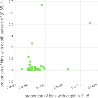
Note that there are 2 samples that are very high on the y-axis. Those correspond to the tan and pink and light-tan colored samples that have variable coverage in the depth plots (in the HTML, this plot is hoverable so those samples are easily discoverable).

Samples that are outliers like this have a coverage bias that will make them problematic for CNV calling and likely other prolems.

Chromosomal Differences

Because indexcov just does a simple per-sample median normalization (and because there are unknown coverage biases) some variation in coverage still remains. This is especially apparent on chromosomes with high-GC content. For example, here is chromosome 19, a high-GC chromosome, for the same 45-member cohort:

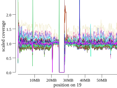
Note that there is extreme coverage variability in all samples, but especially in the tan sample. Don’t mistake variability like this for an event, if you see a sample like that check if it’s high on the bin plot.

(There does appear to be a true homozygous duplication in the rust-colored sample just after the centromere.)

Data Files

indexcov outputs data files (linked from the HTML). One is a ped file that contains all per-sample info:

1. usual pedigree info with -9 for parents
2. X and Y copy-number
3. proportion of bins in and out of 0.85-1.15 range
4. propotion of bins < 0.15
5. slope of cumulative coverage line as it passes through 1.
6. PCs 1 through 5

It also outputs a bed.gz file that an additional column for each sample and rows for each 16KB region in the genome so that users can do their own analyses and visualizations

Use it

If you have whole genomes and haven’t used indexcov, give it a try. You can download a truly static binary here. And run it on a hundred bams in under 2 minutes like this:

goleft indexcov -d output-dir/ /path/to/*.bam

And, if you do use it, please cite the paper